Background

In this post I will cover a few low rank tensor decomposition methods for taking layers in existing deep learning models and making them more compact. I will also share PyTorch code that uses Tensorly for performing CP decomposition and Tucker decomposition of convolutional layers.

Although hopefully most of the post is self contained, a good review of tensor decompositions can be found here. The author of Tensorly also created some really nice notebooks about Tensors basics. That helped me getting started, and I recommend going through that.

Together with pruning, tensor decompositions are practical tools for speeding up existing deep neural networks, and I hope this post will make them a bit more accessible.

张量分解和剪枝一样是用来加速DNN的，张量分解将one layer分解为多个smaller layer，尽管层数增加了，但是整个浮点数操作的数量和权重都会减少。

These methods take a layer and decompose it into several smaller layers. Although there will be more layers after the decomposition, the total number of floating point operations and weights will be smaller. Some reported results are on the order of x8 for entire networks (not aimed at large tasks like imagenet, though), or x4 for specific layers inside imagenet. My experience was that with these decompositions I was able to get a speedup of between x2 to x4, depending on the accuracy drop I was willing to take.

In this blog post I covered a technique called pruning for reducing the number of parameters in a model. Pruning requires making a forward pass (and sometimes a backward pass) on a dataset, and then ranks the neurons according to some criterion on the activations in the network.

上面那个链接里包含了很多剪枝的内容，它提到剪枝需要进行前向传播和后向传播并且对神经元进行排序。而TD支队当前层的权重进行分解，并且它的低秩特点使得他在过拟合的网络上效果最好。

Quite different from that, tensor decomposition methods use only the weights of a layer, with the assumption that the layer is over parameterized and its weights can be represented by a matrix or tensor with a lower rank. This means they work best in cases of over parameterized networks. Networks like VGG are over parameterized by design. Another example of an over parameterized model is fine tuning a network for an easier task with fewer categories.

Similarly to pruning, after the decomposition usually the model needs to be fine tuned to restore accuracy.

和剪枝一样，在分解之后，需要对模型进行微调来恢复精度。但是还有一些缺点

他们对线性关系的layer进行操作（卷积层或全连接层），会忽视这些层之后的非线性关系

忽视不同layer之间的交互

One last thing worth noting before we dive into details, is that while these methods are practical and give nice results, they have a few drawbacks:

They operate on the weights of a linear layer (like a convolution or a fully connected layer), and ignore any non linearity that comes after them.
They are greedy and perform the decomposition layer wise, ignoring interactions between different layers.

There are works that try to address these issues, and its still an active research area.

Truncated SVD for decomposing fully connected layers

The first reference I could find of using this for accelerating deep neural networks, is in the Fast-RCNN paper. Ross Girshick used it to speed up the fully connected layers used for detection. Code for this can be found in the pyfaster-rcnn implementation.

SVD recap

The singular value decomposition lets us decompose any matrix A with n rows and m columns:

$A_{n\times m} = U_{n\times n} S_{n\times m} V^T_{m\times m}$

S is a diagonal matrix with non negative values along its diagonal (the singular values), and is usually constructed such that the singular values are sorted in descending order. U and V are orthogonal matrices: $U^TU=V^TV=I$

If we take the largest $t$ singular values and zero out the rest, we get an approximation of $A$:

$\hat{A} = U_{n\times t}S_{t\times t}V^T_{m\times t}$

截断SVD，具有t秩

$\hat{A}$ has the nice property of being the rank $t$ matrix that has the Frobenius-norm closest to $A$, so $\hat{A}$ is a good approximation of $A$ if $t$ is large enough.

SVD on a fully connected layer

A fully connected layer essentially does matrix multiplication of its input by a matrix A, and then adds a bias b:

$Ax+b$

We can take the SVD of A, and keep only the first t singular values.

$(U_{n\times t}S_{t\times t}V^T_{m\times t})x + b = U_{n\times t} ( S_{t\times t}V^T_{m\times t} x ) + b$

Instead of a single fully connected layer, this guides us how to implement it as two smaller ones:

The first one will have a shape of $m\times t$, will have no bias, and its weights will be taken from $S_{t\times t}V^T$.
The second one will have a shape of $t\times n$, will have a bias equal to b, and its weights will be taken from $U$.

The total number of weights dropped from $n\times m$ to $t(n+m)$.

Tensor decompositions on convolutional layers

A 2D convolutional layer is a multi dimensional matrix (from now on - tensor) with 4 dimensions:

cols x rows x input_channels x output_channels.

filters的大小为cols x rows x input_channels，有output_channels个filters

Following the SVD example, we would want to somehow decompose the tensor into several smaller tensors. The convolutional layer would then be approximated by several smaller convolutional layers.

For this we will use the two popular (well, at least in the world of Tensor algorithms) tensor decompositions: the CP decomposition and the Tucker decomposition (also called higher-order SVD and many other names).

深度学习中不同类型卷积的综合介绍：2D卷积、3D卷积、转置卷积、扩张卷积、可分离卷积、扁平卷积、分组卷积、随机分组卷积、逐点分组卷积等pytorch代码实现和解析

1412.6553 Speeding-up Convolutional Neural Networks Using Fine-tuned CP-Decomposition

_1412.6553 Speeding-up Convolutional Neural Networks Using Fine-tuned CP-Decomposition_ shows how CP-Decomposition can be used to speed up convolutional layers. As we will see, this factors the convolutional layer into something that resembles mobile nets.

They were able to use this to accelerate a network by more than x8 without significant decrease in accuracy. In my own experiments I was able to use this get a x2 speedup on a network based on VGG16 without accuracy drop.

My experience with this method is that the fine tuning learning rate needs to be chosen very carefuly to get it to work, and the learning rate should usually be very small (around $10^{-6}$).

A rank R matrix can be viewed as a sum of R rank 1 matrices, were each rank 1 matrix is a column vector multiplying a row vector: $\sum_1^Ra_i*b_i^T$

The SVD gives us a way for writing this sum for matrices using the columns of U and V from the SVD: $\sum_1^R \sigma_i u_i*v_i^T$.

If we choose an R that is less than the full rank of the matrix, than this sum is just an approximation, like in the case of truncated SVD.

The CP decomposition lets us generalize this for tensors.

Using CP-Decompoisition, our convolutional kernel, a 4 dimensional tensor $K(i, j, s, t)$ can be approximated similarly for a chosen R:

$\sum_{r=1}^R K^x(i,r)K^y(j,r)K^s(s,r)K^t(t,r)$.

We will want R to be small for the decomposition to be effecient, but large enough to keep a high approximation accuracy.

The convolution forward pass with CP Decomposition

To forward the layer, we do convolution with an input $X(i, j, s)$:

$V(x, y, t) = \sum_i \sum_j \sum_sK(i, j, s, t)X(x-i, y-j, s) \\= \sum_r\sum_i \sum_j \sum_sK^x(i,r)K^y(j,r)K^s(s,r)K^t(t,r)X(x-i, y-j, s) \\= \sum_rK^t(t,r) \sum_i \sum_j K^x(i,r)K^y(j,r)\sum_sK^s(s,r)X(x-i, y-j, s)$

This gives us a recipe to do the convolution:

First do a pointwise ($1\times 1\times S$) convolution with $K(s)$. This reduces the number of input channels from S to R. The convolutions will next be done on a smaller number of channels, making them faster.
Perform seperable convolutions in the spatial dimensions with $K^x_r,K^y_r$. Like in mobilenets the convolutions are depthwise seperable, done in each channel separately. Unlike mobilenets the convolutions are also separable in the spatial dimensions.
Do another pointwise convolution to change the number of channels from R to T If the original convolutional layer had a bias, add it at this point.

点卷积（pointwise convolution）
点卷积是一种特殊的卷积运算，他的卷积大小是$1 \times 1$。其作用主要是改变输入数据的通道数channels，在深度学习中用于将高维空间映射到地位空间，而不改变数据的空间维度（宽度和高度）

可分离卷积（separable convolution）
这是一种将常规卷积分解成更小或更易于计算的操作的技术。在深度学习中，最常见的可分离卷积是深度可分离卷积（depthwise separable convolution），它由两个步骤组成：深度卷积（depthwise convolution）和点卷积。

深度卷积: 这一步骤单独对每个输入通道进行卷积操作。这意味着每个通道有一个独立的卷积核，这些卷积核只在其相应的通道上滑动，处理空间信息。

好的，让我们一步一步地了解这个公式，并将其与您之前提到的三个关于卷积操作的观点联系起来。

公式解释：

公式描述了如何使用 CP 分解（Candecomp/Parafac）来执行卷积操作。在这里，原始的卷积核 ( K(i, j, s, t) ) 被分解为更小的成分 ( K^x(i,r) )，( K^y(j,r) )，( K^s(s,r) )，和 ( K^t(t,r) )。

第一部分: ( V(x, y, t) = \sum_i \sum_j \sum_sK(i, j, s, t)X(x-i, y-j, s) )
- 这表示标准的卷积操作，其中 ( K ) 是卷积核，( X ) 是输入特征图，( V ) 是输出特征图。
第二部分: ( = \sum_r\sum_i \sum_j \sum_sK^x(i,r)K^y(j,r)K^s(s,r)K^t(t,r)X(x-i, y-j, s) )
- 这表示 CP 分解的应用。卷积核 ( K ) 被分解为四个部分，分别处理不同的维度（空间和通道）。
第三部分: ( = \sum_rK^t(t,r) \sum_i \sum_j K^x(i,r)K^y(j,r)\sum_sK^s(s,r)X(x-i, y-j, s) )
- 这是将上述分解进一步展开，显示了分解操作是如何整合进卷积计算中的。

关联到三个观点：

点卷积（Pointwise Convolution）:
- 公式中的 ( \sum_sK^s(s,r)X(x-i, y-j, s) ) 代表点卷积。这里，( K^s(s,r) ) 起到了改变通道数量的作用，从 ( S ) 通道减少到 ( R )。
可分离卷积（Separable Convolution）:
- 公式中的 ( \sum_i \sum_j K^x(i,r)K^y(j,r) ) 表示可分离卷积。这里，卷积核被分解为沿 x 和 y 方向的两个独立成分，这减少了计算量。
再次进行点卷积:
- 公式中的 ( \sum_rK^t(t,r) ) 是另一个点卷积步骤。在这一步中，通道数从 ( R ) 再变回原来的 ( T )。这种操作与 MobileNets 中使用的类似，但是由于它是从原始卷积层的分解得来的，因此它可以用于已存在的网络架构。

通过这种方式，CP 分解使得我们可以通过一系列更简单、计算量更小的操作来近似原始的卷积操作。这不仅减少了所需的计算资源，还保持了网络的效能。希望这能帮助您更好地理解这个公式和它与卷积操作之间的联系！如果您还有其他疑问，欢迎继续提问。

Notice the combination of pointwise and depthwise convolutions like in mobilenets. While with mobilenets you have to train a network from scratch to get this structure, here we can decompose an existing layer into this form.

As with mobile nets, to get the most speedup you will need a platform that has an efficient implementation of depthwise separable convolutions.

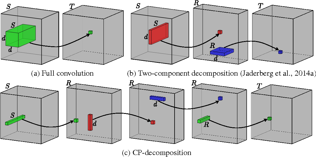_Image taken from the paper. The bottom row is an illustration of the convolution steps after CP-decomposition._

Convolutional layer CP-Decomposition with PyTorch and Tensorly

def cp_decomposition_conv_layer(layer, rank):
    """ Gets a conv layer and a target rank, 
        returns a nn.Sequential object with the decomposition """

    # Perform CP decomposition on the layer weight tensorly. 
    last, first, vertical, horizontal = \
        parafac(layer.weight.data, rank=rank, init='svd')

    pointwise_s_to_r_layer = torch.nn.Conv2d(in_channels=first.shape[0], \
            out_channels=first.shape[1], kernel_size=1, stride=1, padding=0, 
            dilation=layer.dilation, bias=False)

    depthwise_vertical_layer = torch.nn.Conv2d(in_channels=vertical.shape[1], 
            out_channels=vertical.shape[1], kernel_size=(vertical.shape[0], 1),
            stride=1, padding=(layer.padding[0], 0), dilation=layer.dilation,
            groups=vertical.shape[1], bias=False)

    depthwise_horizontal_layer = \
        torch.nn.Conv2d(in_channels=horizontal.shape[1], \
            out_channels=horizontal.shape[1], 
            kernel_size=(1, horizontal.shape[0]), stride=layer.stride,
            padding=(0, layer.padding[0]), 
            dilation=layer.dilation, groups=horizontal.shape[1], bias=False)

    pointwise_r_to_t_layer = torch.nn.Conv2d(in_channels=last.shape[1], \
            out_channels=last.shape[0], kernel_size=1, stride=1,
            padding=0, dilation=layer.dilation, bias=True)

    pointwise_r_to_t_layer.bias.data = layer.bias.data

    depthwise_horizontal_layer.weight.data = \
        torch.transpose(horizontal, 1, 0).unsqueeze(1).unsqueeze(1)
    depthwise_vertical_layer.weight.data = \
        torch.transpose(vertical, 1, 0).unsqueeze(1).unsqueeze(-1)
    pointwise_s_to_r_layer.weight.data = \
        torch.transpose(first, 1, 0).unsqueeze(-1).unsqueeze(-1)
    pointwise_r_to_t_layer.weight.data = last.unsqueeze(-1).unsqueeze(-1)

    new_layers = [pointwise_s_to_r_layer, depthwise_vertical_layer, \
                    depthwise_horizontal_layer, pointwise_r_to_t_layer]
    
    return nn.Sequential(*new_layers)

1511.06530 Compression of Deep Convolutional Neural Networks for Fast and Low Power Mobile Applications

_1511.06530 Compression of Deep Convolutional Neural Networks for Fast and Low Power Mobile Applications_ is a really cool paper that shows how to use the Tucker Decomposition for speeding up convolutional layers with even better results. I also used this accelerate an over-parameterized VGG based network, with better accuracy than CP Decomposition. As the authors note in the paper, it lets us do the finetuning using higher learning rates (I used $10^{-3}$).

The Tucker Decomposition, also known as the higher order SVD (HOSVD) and many other names, is a generalization of SVD for tensors. $K(i, j, s, t) = \sum_{r_1=1}^{R_1}\sum_{r_2=1}^{R_2}\sum_{r_3=1}^{R_3}\sum_{r_4=1}^{R_4}\sigma_{r_1 r_2 r_3 r_4} K^x_{r1}(i)K^y_{r2}(j)K^s_{r3}(s)K^t_{r4}(t)$

The reason its considered a generalization of the SVD is that often the components of $\sigma_{r_1 r_2 r_3 r_4}$ are orthogonal, but this isn’t really important for our purpose. $\sigma_{r_1 r_2 r_3 r_4}$ is called the core matrix, and defines how different axis interact.

In the CP Decomposition described above, the decomposition along the spatial dimensions $K^x_r(i)K^y_r(j)$ caused a spatially separable convolution. The filters are quite small anyway, typically 3x3 or 5x5, so the separable convolution isn’t saving us a lot of computation, and is an aggressive approximation.

The Tucker decomposition has the useful property that it doesn’t have to be decomposed along all the axis (modes). We can perform the decomposition along the input and output channels instead (a mode-2 decomposition):

$K(i, j, s, t) = \sum_{r_3=1}^{R_3}\sum_{r_4=1}^{R_4}\sigma_{i j r_3 r_4}(j)K^s_{r3}(s)K^t_{r4}(t)$

The convolution forward pass with Tucker Decomposition

Like for CP decomposition, lets write the convolution formula and plug in the kernel decomposition:

$V(x, y, t) = \sum_i \sum_j \sum_sK(i, j, s, t)X(x-i, y-j, s)$ $V(x, y, t) = \sum_i \sum_j \sum_s\sum_{r_3=1}^{R_3}\sum_{r_4=1}^{R_4}\sigma_{(i)(j) r_3 r_4}K^s_{r3}(s)K^t_{r4}(t)X(x-i, y-j, s)$ $V(x, y, t) = \sum_i \sum_j \sum_{r_4=1}^{R_4}\sum_{r_3=1}^{R_3}K^t_{r4}(t)\sigma_{(i)(j) r_3 r_4} \sum_s\ K^s_{r3}(s)X(x-i, y-j, s)$

This gives us the following recipe for doing the convolution with Tucker Decomposition:

Point wise convolution with $K^s_{r3}(s)$ for reducing the number of channels from S to $R_3$.
Regular (not separable) convolution with $\sigma_{(i)(j) r_3 r_4}$. Instead of S input channels and T output channels like the original layer had, this convolution has $R_3$ input channels and $R_4$ output channels. If these ranks are smaller than S and T, this is were the reduction comes from.
Pointwise convolution with $K^t_{r4}(t)$ to get back to T output channels like the original convolution. Since this is the last convolution, at this point we add the bias if there is one.

How can we select the ranks for the decomposition ?

One way would be trying different values and checking the accuracy. I played with heuristics like $R_3 = S/3$ , $R_4 = T/3$ with good results.

_Ideally selecting the ranks should be automated._

The authors suggested using variational Bayesian matrix factorization (VBMF) (Nakajima et al., 2013) as a method for estimating the rank.

VBMF is complicated and is out of the scope of this post, but in a really high level summary what they do is approximate a matrix $V_{LxM}$ as the sum of a lower ranking matrix $B_{LxH}A^T_{HxM}$ and gaussian noise. After A and B are found, H is an upper bound on the rank.

To use this for tucker decomposition, we can unfold the s and t components of the original weight tensor to create matrices. Then we can estimate $R_3$ and $R_4$ as the rank of the matrices using VBMF.

I used this python implementation of VBMF and got convinced it works :-)

VBMF usually returned ranks very close to what I previously found with careful and tedious manual tuning.

This could also be used for estimating the rank for Truncated SVD acceleration of fully connected layers.

Convolutional layer Tucker-Decomposition with PyTorch and Tensorly

def estimate_ranks(layer):
    """ Unfold the 2 modes of the Tensor the decomposition will 
    be performed on, and estimates the ranks of the matrices using VBMF 
    """

    weights = layer.weight.data.numpy()
    unfold_0 = tensorly.base.unfold(weights, 0) 
    unfold_1 = tensorly.base.unfold(weights, 1)
    _, diag_0, _, _ = VBMF.EVBMF(unfold_0)
    _, diag_1, _, _ = VBMF.EVBMF(unfold_1)
    ranks = [diag_0.shape[0], diag_1.shape[1]]
    return ranks

def tucker_decomposition_conv_layer(layer):
    """ Gets a conv layer, 
        returns a nn.Sequential object with the Tucker decomposition.
        The ranks are estimated with a Python implementation of VBMF
        https://github.com/CasvandenBogaard/VBMF
    """

    ranks = estimate_ranks(layer)
    print(layer, "VBMF Estimated ranks", ranks)
    core, [last, first] = \
        partial_tucker(layer.weight.data, \
            modes=[0, 1], ranks=ranks, init='svd')

    # A pointwise convolution that reduces the channels from S to R3
    first_layer = torch.nn.Conv2d(in_channels=first.shape[0], \
            out_channels=first.shape[1], kernel_size=1,
            stride=1, padding=0, dilation=layer.dilation, bias=False)

    # A regular 2D convolution layer with R3 input channels 
    # and R3 output channels
    core_layer = torch.nn.Conv2d(in_channels=core.shape[1], \
            out_channels=core.shape[0], kernel_size=layer.kernel_size,
            stride=layer.stride, padding=layer.padding, dilation=layer.dilation,
            bias=False)

    # A pointwise convolution that increases the channels from R4 to T
    last_layer = torch.nn.Conv2d(in_channels=last.shape[1], \
        out_channels=last.shape[0], kernel_size=1, stride=1,
        padding=0, dilation=layer.dilation, bias=True)

    last_layer.bias.data = layer.bias.data

    first_layer.weight.data = \
        torch.transpose(first, 1, 0).unsqueeze(-1).unsqueeze(-1)
    last_layer.weight.data = last.unsqueeze(-1).unsqueeze(-1)
    core_layer.weight.data = core

    new_layers = [first_layer, core_layer, last_layer]
    return nn.Sequential(*new_layers)

Summary

In this post we went over a few tensor decomposition methods for accelerating layers in deep neural networks.

Truncated SVD can be used for accelerating fully connected layers.
CP Decomposition decomposes convolutional layers into something that resembles mobile-nets, although it is even more aggressive since it is also separable in the spatial dimensions.
Tucker Decomposition reduced the number of input and output channels the 2D convolution layer operated on, and used pointwise convolutions to switch the number of channels before and after the 2D convolution.

I think it’s interesting how common patterns in network design, pointwise and depthwise convolutions, naturally appear in these decompositions!

upupwords

张量分解与深度学习